A recap of our model
Our model is a simple OLS with 4 predictors and an intercept.
\[ \text{pv2p} = \beta_0 + \beta_1 \cdot \text{G2GDP} + \beta_2 \cdot \text{NETAPP} + \beta_3 \cdot \text{TERM1INC} + \beta_4 \cdot \text{LAG} \]
Where:
| Variable | Explanation |
|---|---|
| \(\text{pv2p}\) | State-level incumbent party pv2p |
| \(\text{G2GDP}\) | State-level Q2 GDP growth |
| \(\text{NETAPP}\) | State-level two-candidate poll |
| \(\text{TERM1INC}\) | Sitting president? |
| \(\text{LAG}\) | State-level previous election pv2p |
We predicted a Trump win with 312 against 226 electoral votes. Here are the actual results pv2p and the prediction preds.
##    POLL Q2GDP   SIT  LAG swing          state pv2p preds
## 1  37.7   4.8 FALSE 39.3     0           Utah 39.0  34.7
## 2  40.3   3.2 FALSE 41.6     0        Montana 39.7  37.6
## 3  41.2   5.3 FALSE 40.2     0       Nebraska 39.4  37.7
## 4  41.1   2.8 FALSE 41.8     0        Indiana 40.4  38.4
## 5  42.7   3.9 FALSE 42.2     0       Missouri 40.6  39.7
## 6  43.6   4.5 FALSE 44.1     0 South Carolina 40.9  40.9
## 7  45.5   3.4 FALSE 45.9     0           Ohio 44.3  43.1
## 8  45.9   2.8 FALSE 47.2     0          Texas 43.0  43.8
## 9  46.5   3.2 FALSE 48.3     0        Florida 43.4  44.6
## 10 48.6   3.1 FALSE 50.2     1        Arizona 47.2  46.9
## 11 49.3   3.5 FALSE 49.3     1 North Carolina 48.4  47.2
## 12 49.2   3.5 FALSE 50.1     1        Georgia 48.9  47.3
## 13 49.9   3.2 FALSE 50.6     1   Pennsylvania 49.1  48.0
## 14 49.7   1.8 FALSE 51.2     1         Nevada 48.4  48.2
## 15 50.4   4.2 FALSE 50.3     1      Wisconsin 49.6  48.2
## 16 50.4   4.2 FALSE 51.4     1       Michigan 49.3  48.6
## 17 52.5   2.1 FALSE 53.7     0  New Hampshire 51.4  51.2
## 18 53.0   1.3 FALSE 53.6     0      Minnesota 52.2  51.6
## 19 53.3   3.2 FALSE 55.2     0       Virginia 52.6  52.2
## 20 53.5   1.7 FALSE 55.5     0     New Mexico 53.1  52.6
## 21 55.8   2.7 FALSE 56.9     0       Colorado 55.6  54.7
## 22 58.7   3.8 FALSE 61.7     0       New York 55.9  58.4
## 23 60.3   2.2 FALSE 59.9     0     Washington 59.6  59.2
## 24 62.8   2.8 FALSE 64.9     0     California 60.7  62.7
## 25 64.3   1.9 FALSE 67.1     0  Massachusetts 62.7  64.6
## 26 64.8   2.3 FALSE 67.0     0       Maryland 64.1  65.0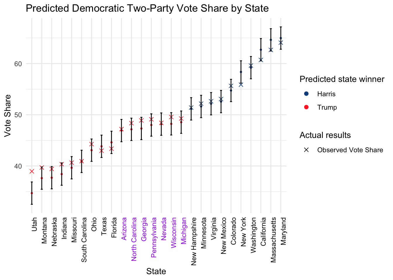
Most of the actual results fall within the 95% confidence interval. We note that states at the far end of the spectrum like Utah and Montana on the left and Massachusetts and Maryland on the right has a systematic regression towards the mean. This could mean that our model works best for tight races and the linear coefficients don’t hold too well for strongholds. Call this Problem A which we will address later in a section. The model overestimates the support for the strongholds on both sides.
Note that within swing states, Harris overperformed our predictions across the board.
Here is the test RMSE for 2024
## [1] 1.493748It can be interpreted that the actual results are within 1.5% vote share difference with our predictions.
National bias
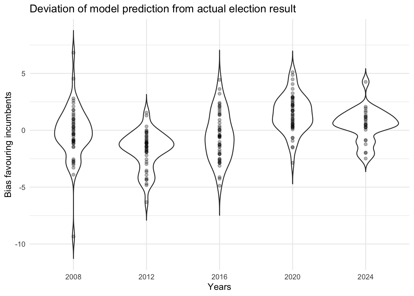
I am also interested to investigate whether the error for each state is correlated in each election. If that’s the case, that will make predictions harder since nice theoretical assumptions don’t hold anymore, and the election results will be severely different from our forecasts if every state swings towards the same direction instead random swings whose effects cancel each other out.
Here each dot represents a state and how much the model prediction is biased from the actual result. We see that on 2008 and 2016 the spread is centered around 0, indicating unbiasedness, while in 2012 the model had a national bias underestimating the incumbent (Obama) while in 2020 the model overestimated Trump and in 2024 it slightly overestimated Harris. Importantly, notice that the bias of each state swings together. This is important because it tells us that the bias is correlated across states in the same year.
Are certain states perculiar?
Let’s see if there is any state that we consistently miss using our model.
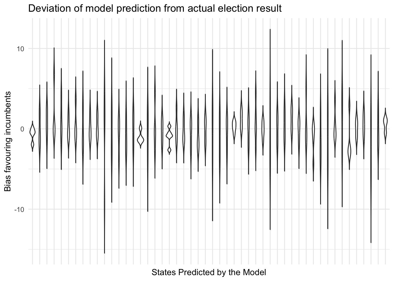
The plot shows that there are no states where we systematically overestimate or underestimate the incumbent over the years.
GDP growth is bad for the incumbent?
Here are the coefficients for our final model
##
## Call:
## lm(formula = pv2p ~ POLL + Q2GDP + SIT + LAG, data = filter(all_data,
##     year != 2024))
##
## Residuals:
##     Min      1Q  Median      3Q     Max
## -8.2544 -0.9846  0.0430  1.1962  6.7362
##
## Coefficients:
##             Estimate Std. Error t value Pr(>|t|)
## (Intercept) -6.73854    0.75357  -8.942 3.29e-16 ***
## POLL         0.78661    0.04331  18.164  < 2e-16 ***
## Q2GDP       -0.10465    0.02859  -3.660 0.000326 ***
## SITTRUE      2.26164    0.30019   7.534 1.91e-12 ***
## LAG          0.31320    0.03980   7.869 2.59e-13 ***
## ---
## Signif. codes:  0 '***' 0.001 '**' 0.01 '*' 0.05 '.' 0.1 ' ' 1
##
## Residual standard error: 1.904 on 191 degrees of freedom
## Multiple R-squared:  0.9676,	Adjusted R-squared:  0.9669
## F-statistic:  1425 on 4 and 191 DF,  p-value: < 2.2e-16
Notice that the coefficient for the GDP is negative. I suppose that this is because there is multi-colinearity among the predictors, which can result in the model to attribute some of the effects from the GDP to another closely associated predictor. Let’s compute the Variance Inflation Factor (VIF) to check whether any values are greater than 10.
##     POLL    Q2GDP      SIT      LAG
## 8.551113 1.207070 1.217843 8.525566
Although GDP was not, it shows that POLL and LAG are closely associated. Let’s look at the pairwise correlation.
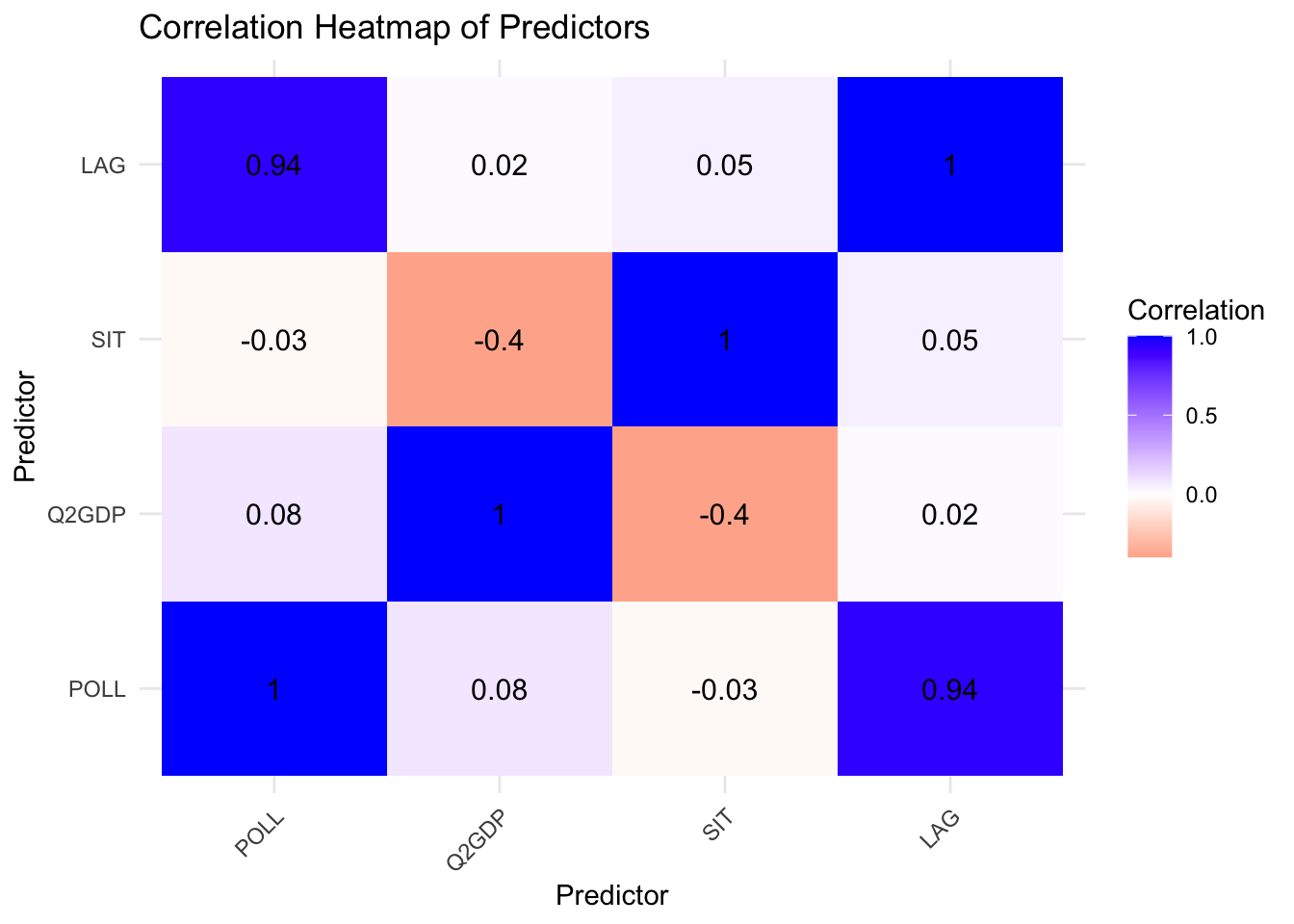
Since there is high correlation between LAG and POLL, we have to employ penalization. Call this Problem B.
Addressing the problems
Problem A
We first try to solve problem A by applying transformations. The linear model output doesn’t limit to between 0 and 1, so we can attempt using a logistic regression instead.
## RMSE (linear): 1.493748## RMSE (logit): 1.564289Logit transformation doesn’t help. If we have more time, I would like to explore possible transformations so that the regression will output values between 0 to 1 and has better performance than our current model.
Problem B
We will apply penalization via ridge regression as an experiment. The test data is 2024 and the train data are the 2008 to 2020 elections. We will scan through the penalty coefficient from \(0.001\) to \(100\).
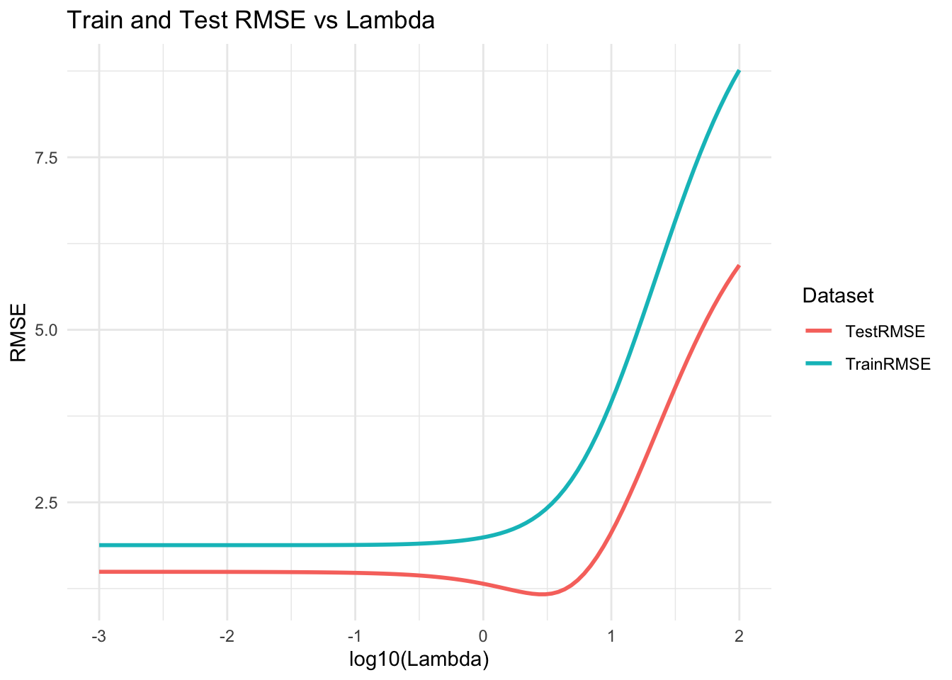
Regularization works. The attentive reader might point out that the test RMSE is consistently lower than the train RMSE, but this is ok as a proof of concept and it might be the case that the 2024 election is more predictable than the others.
## Minimum 2024 RMSE is 1.167115## Chosen lambda is 2.718588The new model has a lower RMSE than our model.
Here are the coefficients (the variables are standardized)
## 5 x 1 sparse Matrix of class "dgCMatrix"
##                     s0
## (Intercept) 48.3259961
## POLL         4.8263366
## Q2GDP       -0.3717357
## LAG          4.1150848
## SIT          1.7147598
Unfortunately, the negative GDP situation is still there. Here are the predictions of the new model.
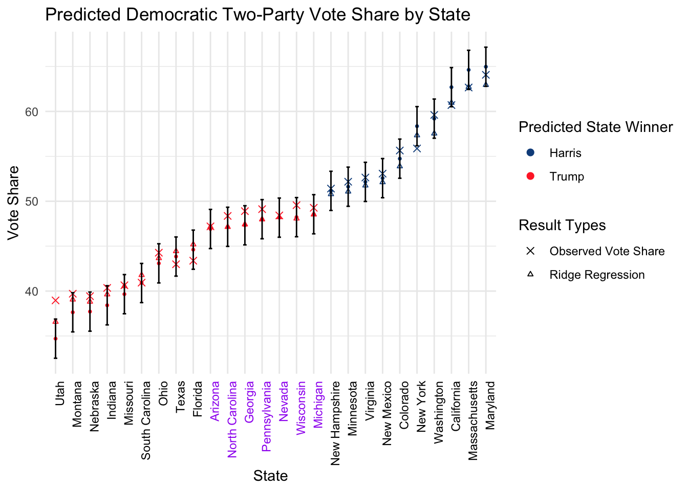
Note that the ridge regression performed better than our model by making better predictions for the stronghold states, while the prediction for the swing states are relatively unchanged. In this case, we have also found a partial solution towards Problem A.
If we have more time, I would like to do a full-fledged model regularization, while incorporating a scheme where the training data and test data are partitioned by random years as batches. This will possibly yield a stronger model and likely solve the negative GDP problem.