Model prediction
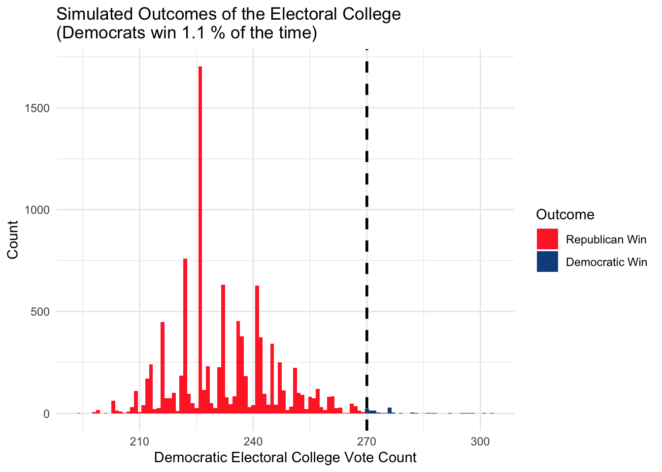
The model predicts a Trump win with 312 against 226, sweeping all seven swing states. See the section below on “Detailed Model Prediction and Model Uncertainty” for the predicted vote share of each state.

Model description
Our final model predicts the electoral college winner by running a simple linear regression to predict the popular vote winner in each state.
\[ \text{pv2p} = \beta_0 + \beta_1 \cdot \text{Q2GDP} + \beta_2 \cdot \text{POLL} + \beta_3 \cdot \text{SIT} + \beta_4 \cdot \text{LAG} \]
Where:
| Variable | Explanation |
|---|---|
| \(\text{pv2p}\) | State-level incumbent party pv2p |
| \(\text{Q2GDP}\) | State-level Q2 GDP growth |
| \(\text{POLL}\) | State-level two-candidate poll |
| \(\text{SIT}\) | Sitting president? |
| \(\text{LAG}\) | State-level previous election pv2p |
Restricted by data availability, our training data includes 196 state-level election results from 2008, 2012, 2016, and 2020.
Model Justification
The regression is an ordinary least-squares (OLS). The model has its origins in Abramowitz’s Time for Change model. Each variable provides perpendicular information on factors driving the popular vote. The GDP informs the economic fundamentals. The poll reflects current voter sentiment. The sitting president flag encodes the incumbency effect. The previous election results provides information on political calcification of each state.
Model coefficients
##
## Call:
## lm(formula = pv2p ~ Q2GDP + POLL + SIT + LAG, data = state_popvote_gdp_polls)
##
## Residuals:
##     Min      1Q  Median      3Q     Max
## -8.2544 -0.9846  0.0430  1.1962  6.7362
##
## Coefficients:
##             Estimate Std. Error t value Pr(>|t|)
## (Intercept) -6.73854    0.75357  -8.942 3.29e-16 ***
## Q2GDP       -0.10465    0.02859  -3.660 0.000326 ***
## POLL         0.78661    0.04331  18.164  < 2e-16 ***
## SITTRUE      2.26164    0.30019   7.534 1.91e-12 ***
## LAG          0.31320    0.03980   7.869 2.59e-13 ***
## ---
## Signif. codes:  0 '***' 0.001 '**' 0.01 '*' 0.05 '.' 0.1 ' ' 1
##
## Residual standard error: 1.904 on 191 degrees of freedom
## Multiple R-squared:  0.9676,	Adjusted R-squared:  0.9669
## F-statistic:  1425 on 4 and 191 DF,  p-value: < 2.2e-16
Model intrepretation
GDP: an estimate of -0.10465 suggest that a 1% higher Q2 GDP growth rate is associated with -0.1% change in vote share.
Polls: an estimate of 0.78661 suggest that a 1% increase in polls is associated with a +0.8% change in vote share.
Incumbency: an estimate of 2.26164 suggest that an incumbent president gets a +2.3% increase in vote share.
Previous election: an estimate of 0.31320 suggest that every 1% of the vote share from the previous election translates to +0.3% to the current election.
Model validation
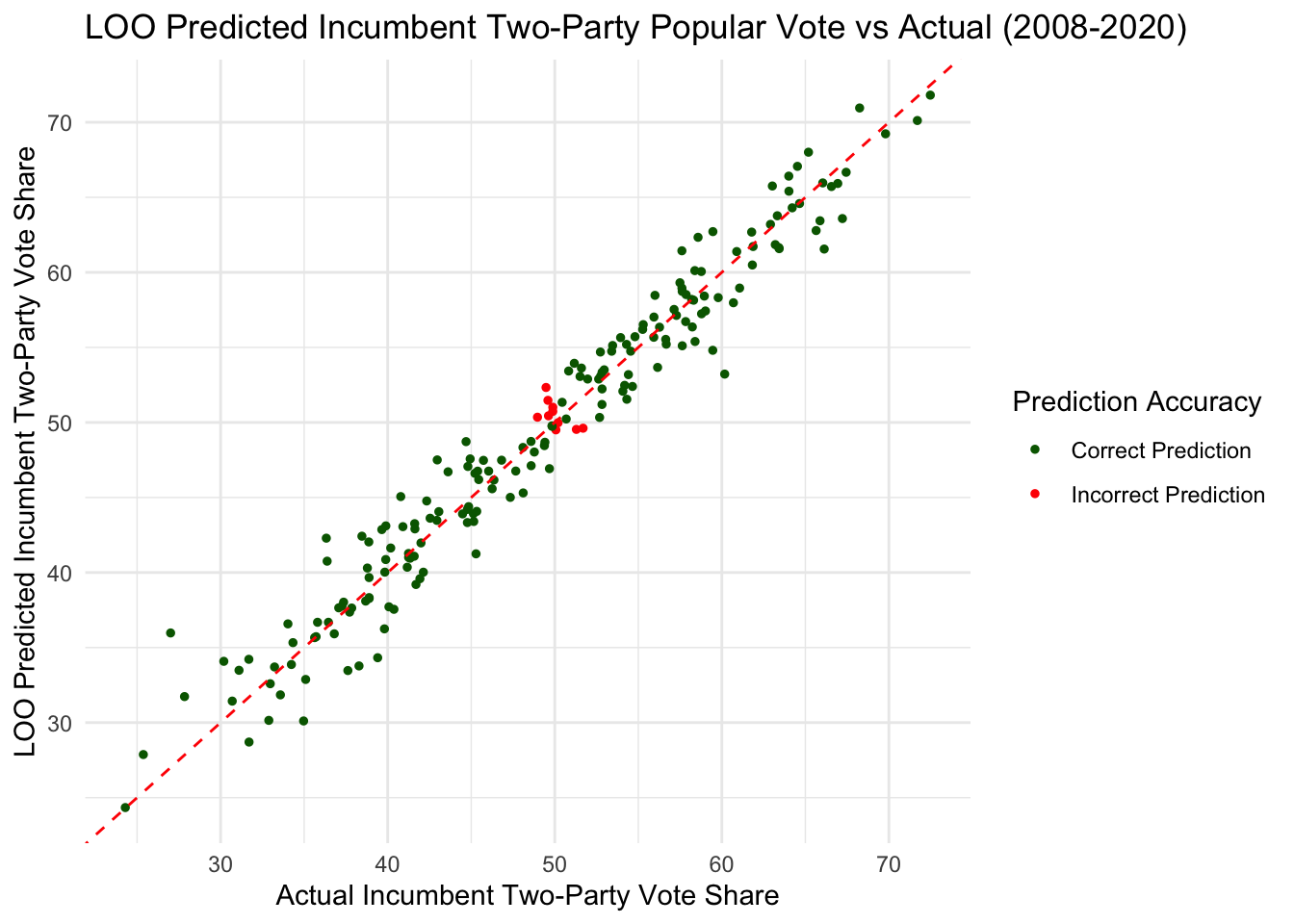
Our in-sample root mean-squared error (RMSE) is given below.
## In-sample RMSE: 1.88Our leave-one-out (LOO) RMSE is given below.
## LOO RMSE: 2.18## LOO RMSE (swing states): 2.11Here we present a plot showing the LOO performance of the model.
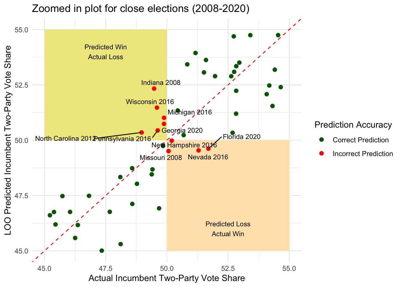
We also verified the OLS assumptions. See appendix below for details
Detailed Model Prediction and Model Uncertainty
Here are the predictors for 2024 and the corresponding incumbent vote share prediction. Swing states are marked. We also include the 95% prediction interval. Numbers are rounded to 2 decimal points for display.
##     POLL Q2GDP   SIT   LAG swing          state preds lower upper
## 1  37.67   4.8 FALSE 39.31     0           Utah 34.70 30.91 38.50
## 2  40.27   3.2 FALSE 41.60     0        Montana 37.63 33.85 41.42
## 3  41.21   5.3 FALSE 40.22     0       Nebraska 37.71 33.92 41.51
## 4  41.13   2.8 FALSE 41.80     0        Indiana 38.42 34.63 42.20
## 5  42.71   3.9 FALSE 42.16     0       Missouri 39.65 35.87 43.44
## 6  43.61   4.5 FALSE 44.07     0 South Carolina 40.89 37.11 44.68
## 7  45.51   3.4 FALSE 45.92     0           Ohio 43.09 39.31 46.87
## 8  45.90   2.8 FALSE 47.17     0          Texas 43.84 40.07 47.62
## 9  46.47   3.2 FALSE 48.31     0        Florida 44.61 40.83 48.38
## 10 48.65   3.1 FALSE 50.16     1        Arizona 46.91 43.14 50.69
## 11 49.34   3.5 FALSE 49.32     1 North Carolina 47.15 43.37 50.93
## 12 49.24   3.5 FALSE 50.12     1        Georgia 47.32 43.54 51.10
## 13 49.87   3.2 FALSE 50.59     1   Pennsylvania 48.00 44.22 51.78
## 14 49.65   1.8 FALSE 51.22     1         Nevada 48.17 44.40 51.95
## 15 50.40   4.2 FALSE 50.32     1      Wisconsin 48.23 44.45 52.01
## 16 50.38   4.2 FALSE 51.41     1       Michigan 48.55 44.77 52.33
## 17 52.48   2.1 FALSE 53.75     0  New Hampshire 51.16 47.38 54.93
## 18 53.00   1.3 FALSE 53.64     0      Minnesota 51.62 47.84 55.40
## 19 53.33   3.2 FALSE 55.15     0       Virginia 52.15 48.38 55.93
## 20 53.52   1.7 FALSE 55.52     0     New Mexico 52.57 48.79 56.35
## 21 55.84   2.7 FALSE 56.94     0       Colorado 54.74 50.96 58.52
## 22 58.69   3.8 FALSE 61.72     0       New York 58.36 54.57 62.14
## 23 60.25   2.2 FALSE 59.93     0     Washington 59.20 55.40 62.99
## 24 62.80   2.8 FALSE 64.91     0     California 62.70 58.90 66.49
## 25 64.25   1.9 FALSE 67.12     0  Massachusetts 64.62 60.82 68.42
## 26 64.78   2.3 FALSE 67.03     0       Maryland 64.97 61.17 68.77
Swing states below are marked in purple. The error bar corresponds to the 95% prediction interval.
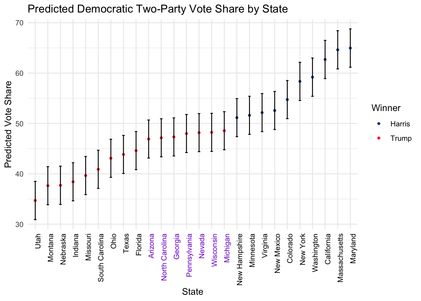
OLS also allows us to fit a distribution on the vote share of the states. This allows us to find the probability of a Harris win as shown below.
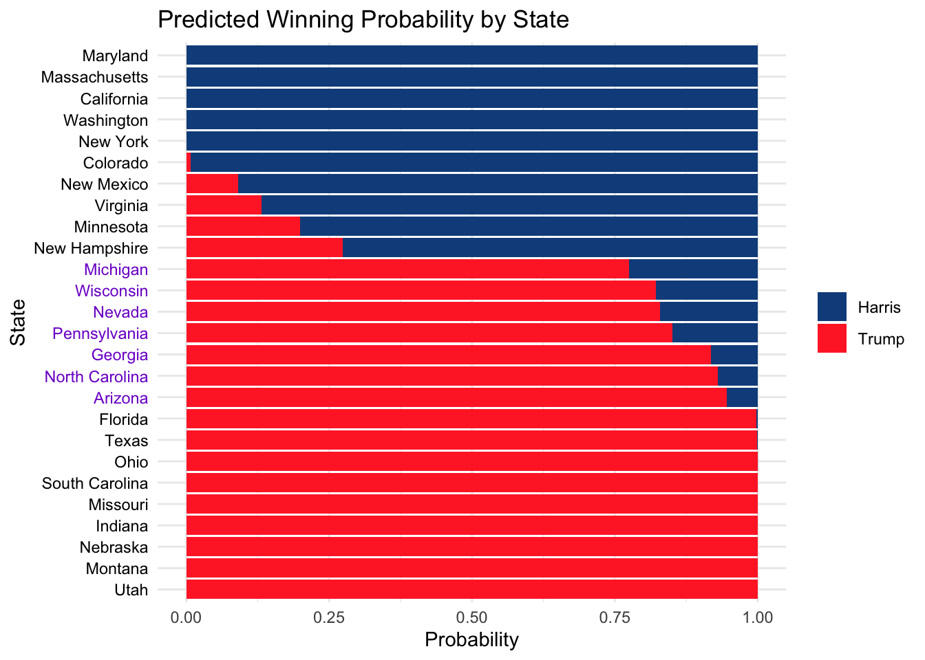
We can then sample from this distribution to get a distribution on the electoral college. Some states are not predicted in our model because polling data is unavailable. Those states are expected to be solid states of either Democrats or Republicans (e.g. Cook’s Political Report), so we will assume for these states that the expert forecasts are correct.
Betting odds
We compare our model prediction to the odds scrapped from the betting market Kalshi on October 28 2024.
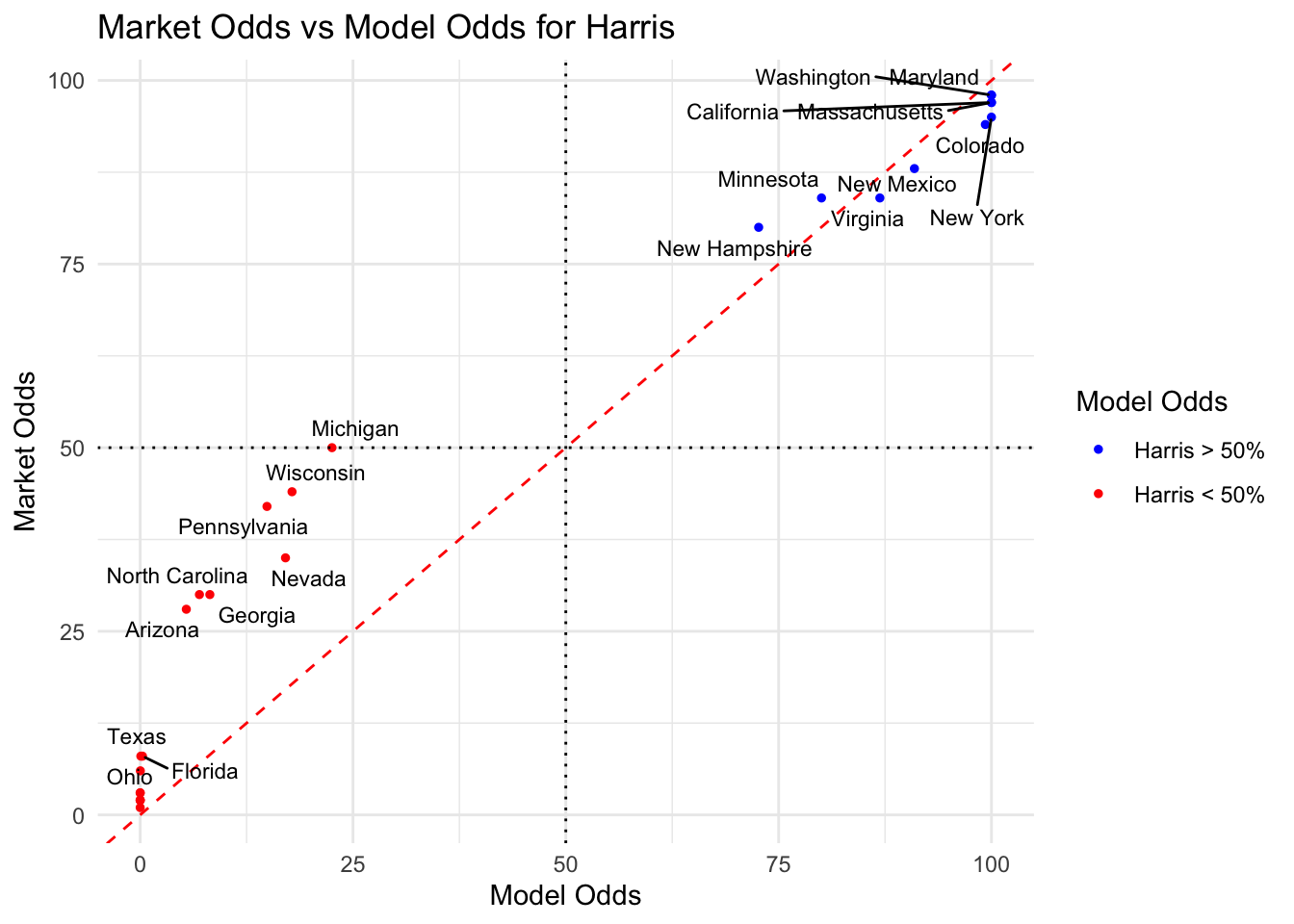
The market shows good fit to non swing-states, including New Hampshire and Minnesota. According to our model, the market overvalues a Harris win in the swing state. This might also suggest that our model underestimate the chances of a Harris win in the swing states.
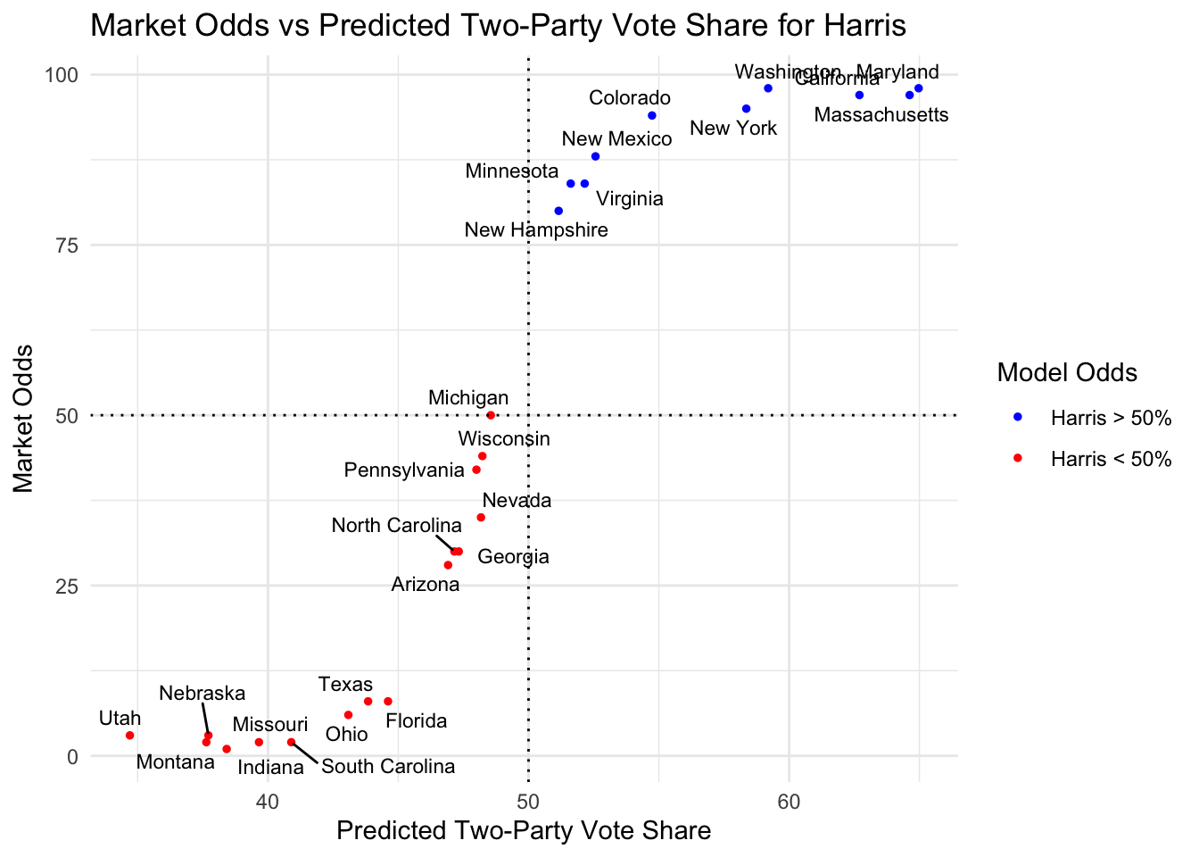
We also plot the model’s predicted vote share against the market odds and note the sigmoid shape.
Appendix
We verify the OLS assumptions
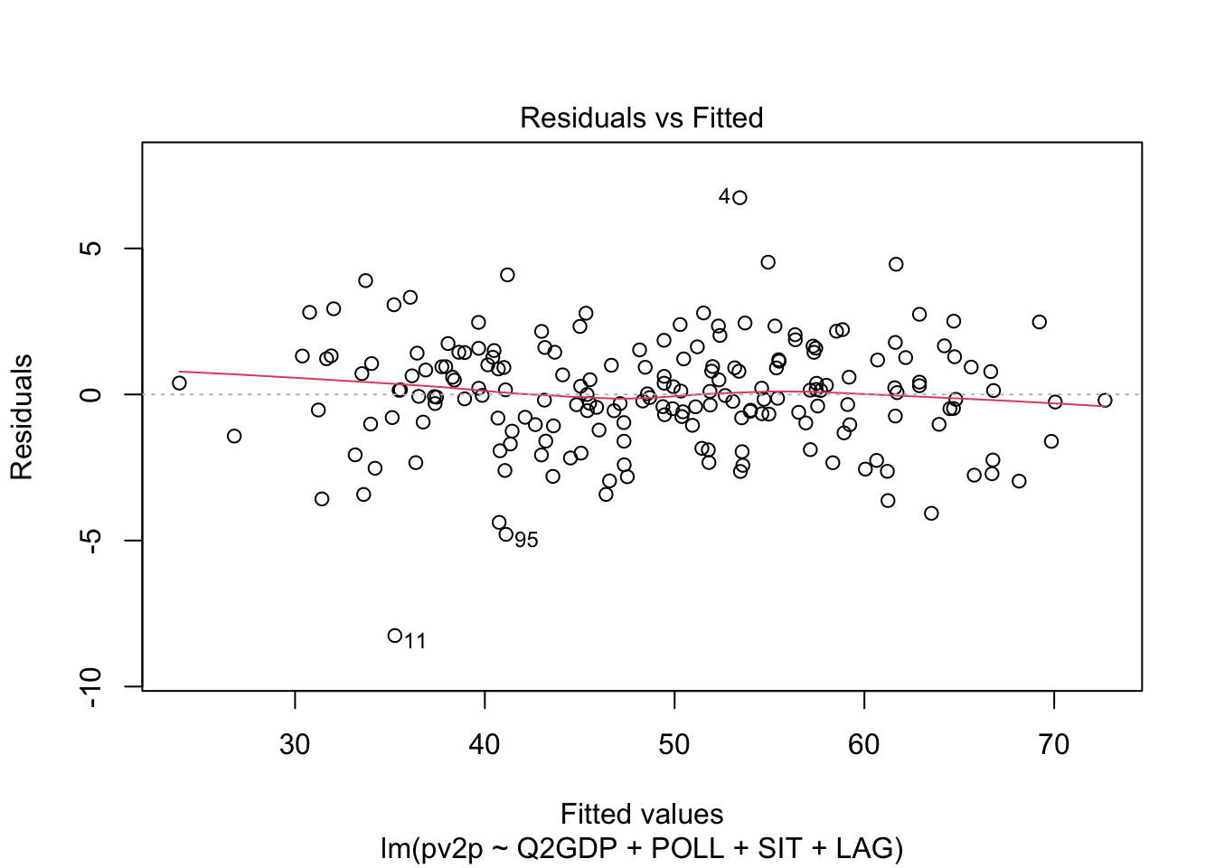
The flat red line shows that linearity holds.
The constant dispersion of values regardless of fitted values shows that homogeneity of residual variance holds.
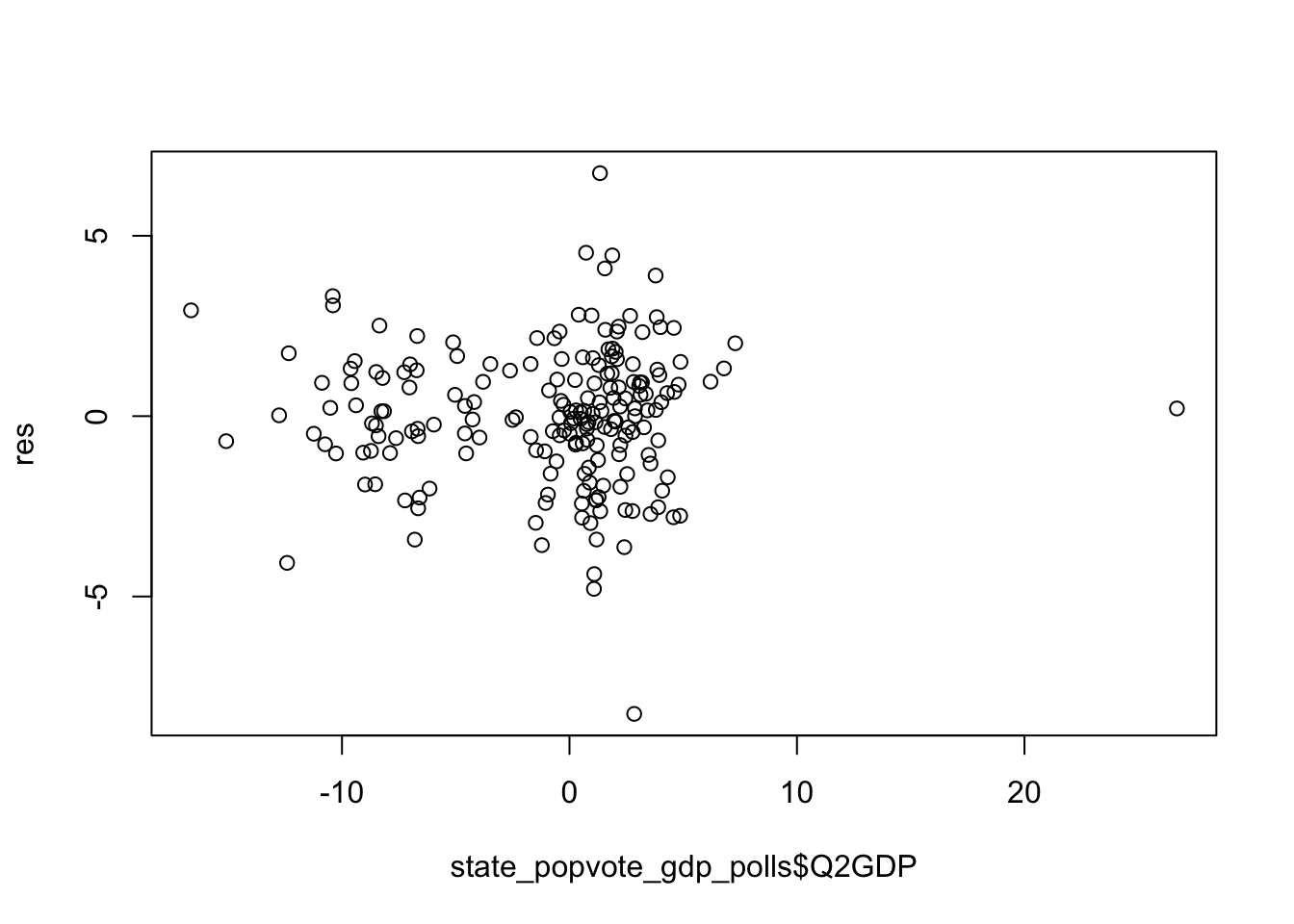
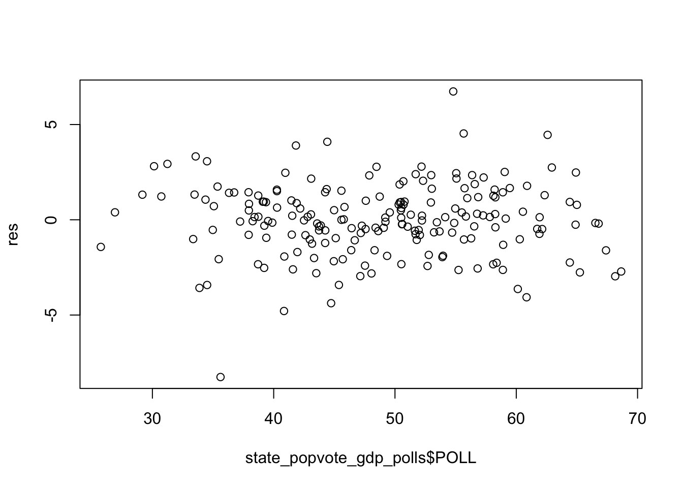
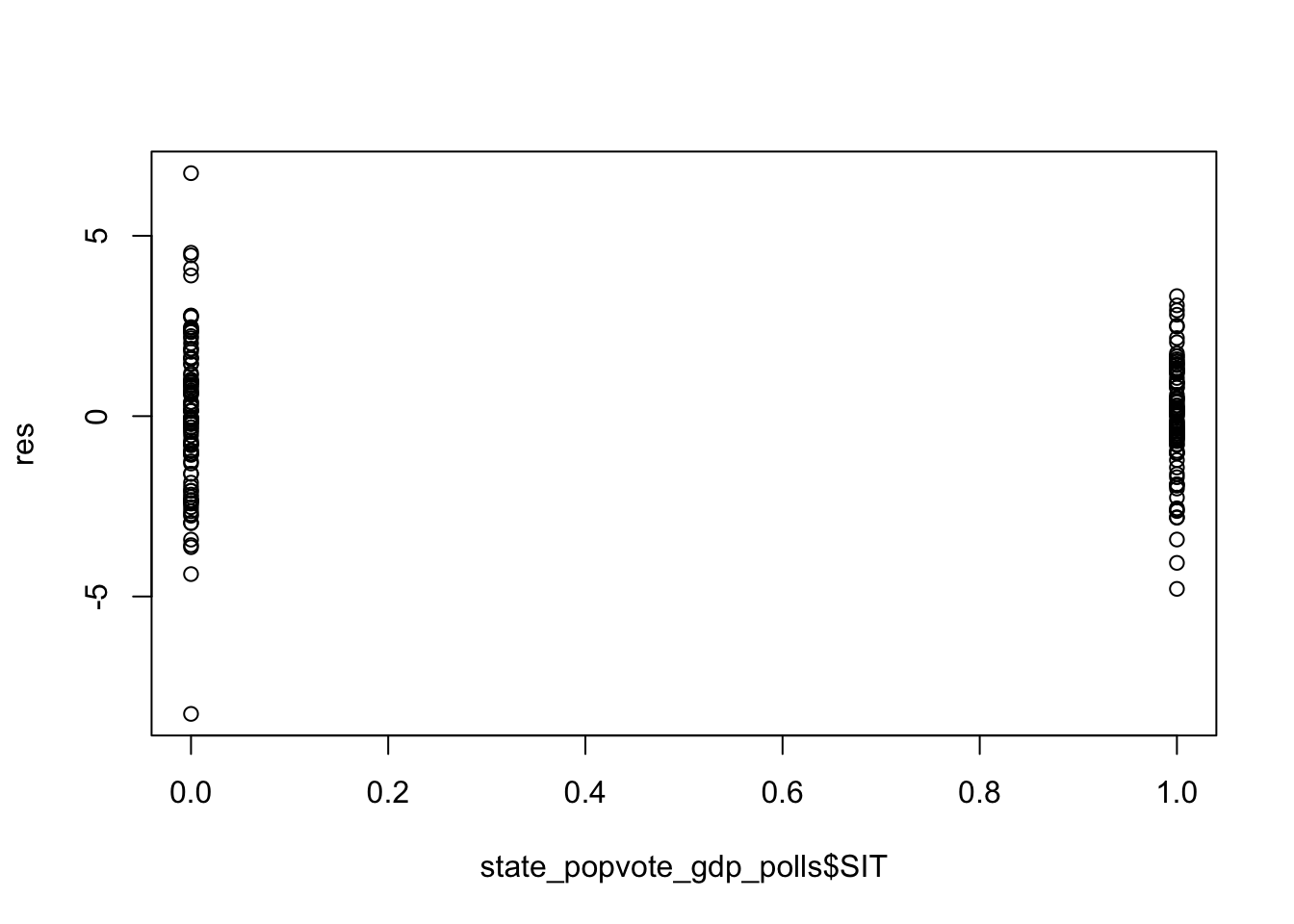
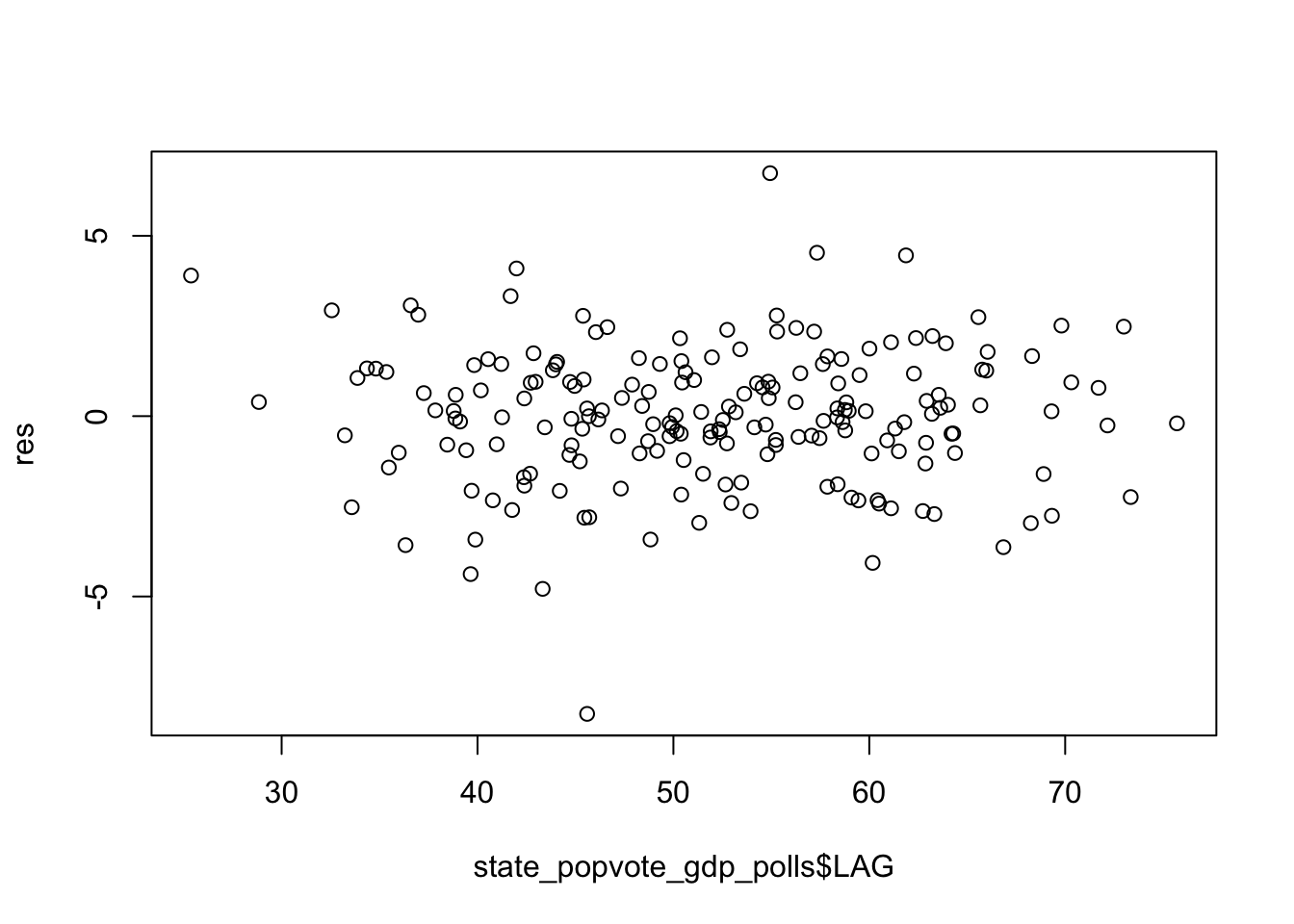
The following plots show constant variance of residuals regardless of predictor values, showing independence.
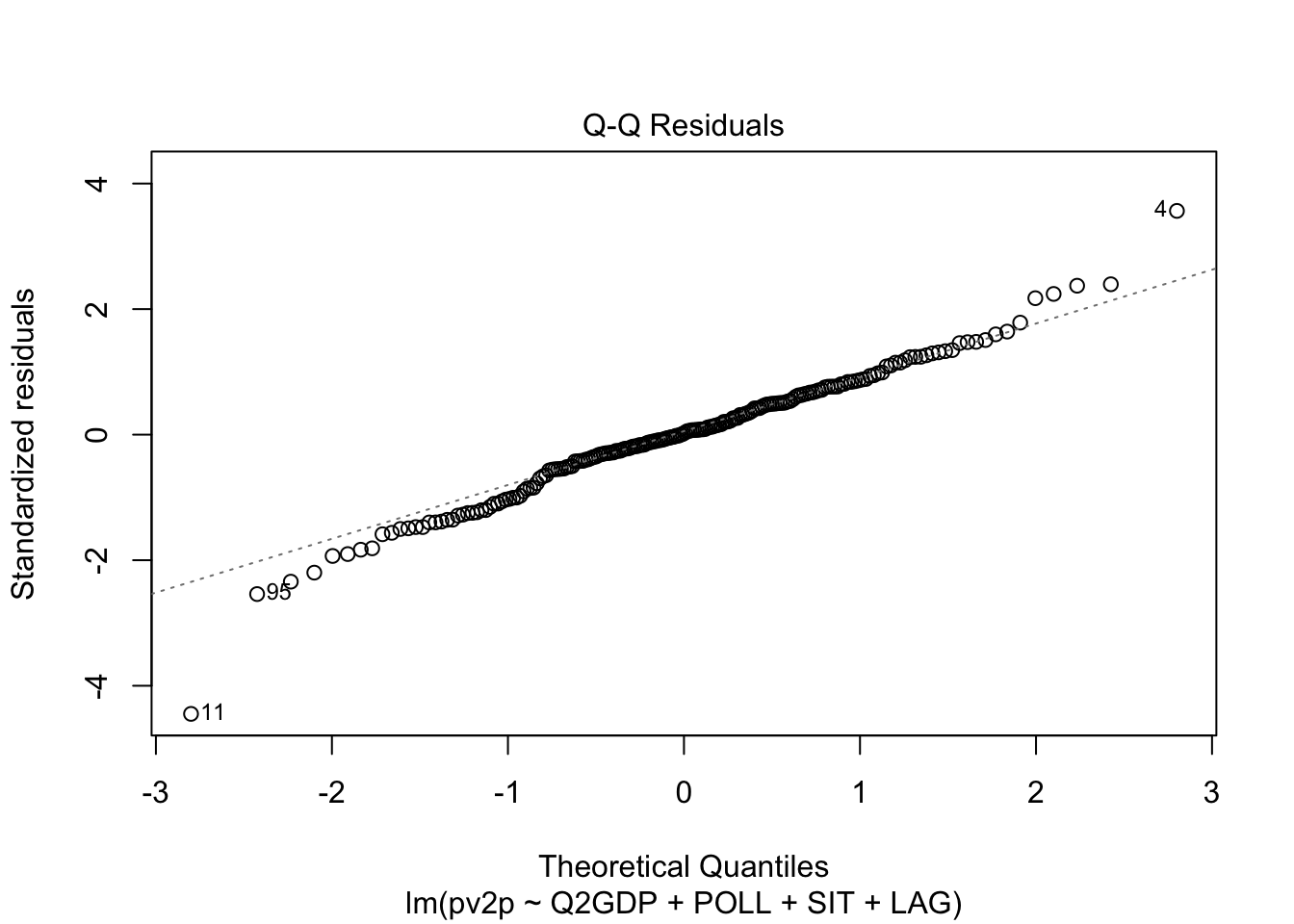
The Q-Q plot below shows that normality holds.
