In this week, we will finalize a model and test whether adding campaign ad spending will improve the model. Recall Abramowitz’s model from the incumbency blog post.
\[ \underbrace{\text{pv2p}}_{\text{incumbent party}} = \beta_0 + \beta_1 \cdot \underbrace{\text{G2GDP}}_{\text{Q2 GDP growth}} + \beta_2 \cdot \underbrace{\text{NETAPP}}_{\text{June Gallup job approval}} + \beta_3 \cdot \underbrace{\text{TERM1INC}}_{\text{sitting pres}} \]
This model achieved a leave-one-out RMSE (LOO-RMSE) of 4.183061 (the lower the better). With Harris and Trump running the race, let’s look at the LOO-RMSE for elections where non-incumbents faced each other.
## Number of non-incumbents elections in database: 7## LOO-RMSE (non-incumbents): 2.711986The LOO-RMSE is lower at 2.7, which is reassuring.
Since Biden dropped out on July 21 and Harris won the nomination on August 5, it might be more accurate for this election to use Q3 GDP growth instead of Q2. Let’s see whether using this metric changes the model’s historical performance by much.
## LOO-RMSE (total): 4.694096## LOO-RMSE (non-incumbents): 3.147468Interestingly, using Q3 data, which is closer to the election date, has a higher RMSE than using Q2 data. However, for most elections, the candidates are known during Q2. Harris was finalized as the candidate during Q3, so for this election, we will proceed with Q3 data, noting but accepting the higher RMSE.
Similarly, let’s use the September Gallup job approval instead of June. Note that this approval rating is still for Biden. I have scrapped the data off this website, with 11 elections from 1980 having consistent September polls. Here are the model’s performance for those 11 elections
## LOO-RMSE (June, total): 4.335228## LOO-RMSE (June, non-incumbents): 5.644492## LOO-RMSE (September, total): 4.519241## LOO-RMSE (September, non-incumbents): 4.081196The same pattern from using Q3 GDP growth occurred, where the RMSE for all elections increased (here from 4.33 to 4.52), while the RMSE for the non-incumbent elections decreased (here from 5.64 to 4.08).
Let’s combine both modifications of using Q3 GDP growth and September Gallup approval ratings, and using the smaller subset of the 11 elections since 1980 where we have September Gallup data.
## LOO-RMSE (Q3, September, total): 6.272696## LOO-RMSE (Q3, September, non-incumbents): 4.470664We achieved a LOO-RMSE of 6.27 generally and 4.47 for non-incumbent elections.
Note that we have been predicting the national two-party vote share. Currently, this national popular vote share doesn’t have much weight since the electoral collage determines who wins. Let’s get more granular and apply this model at the state-level then. We are only interested in recent competitive states. Let’s take a look at the past 3 elections.
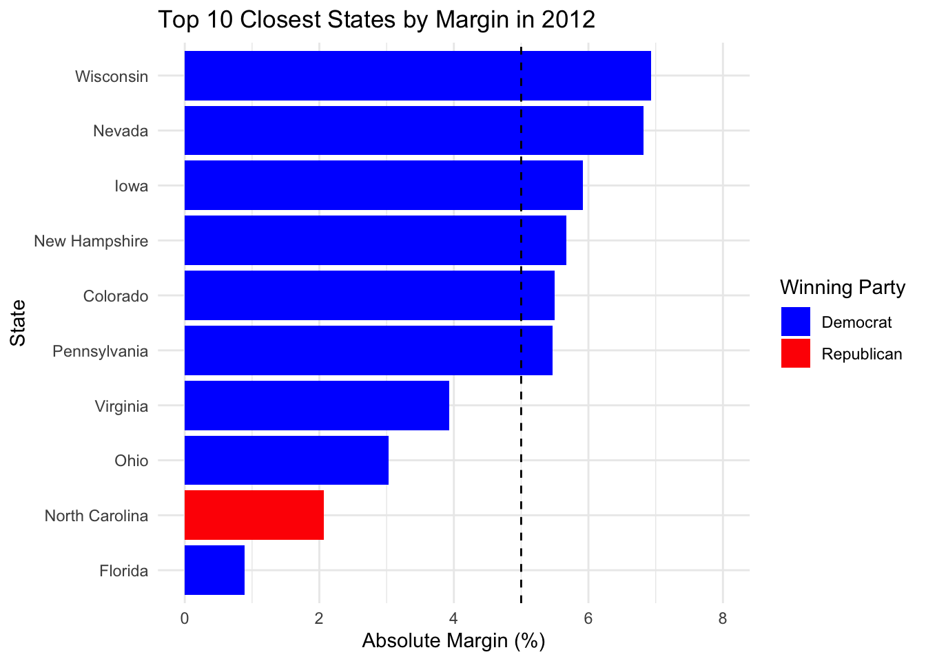
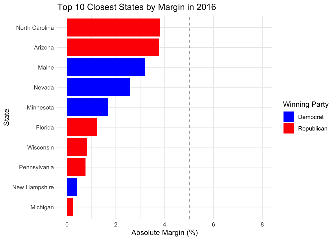
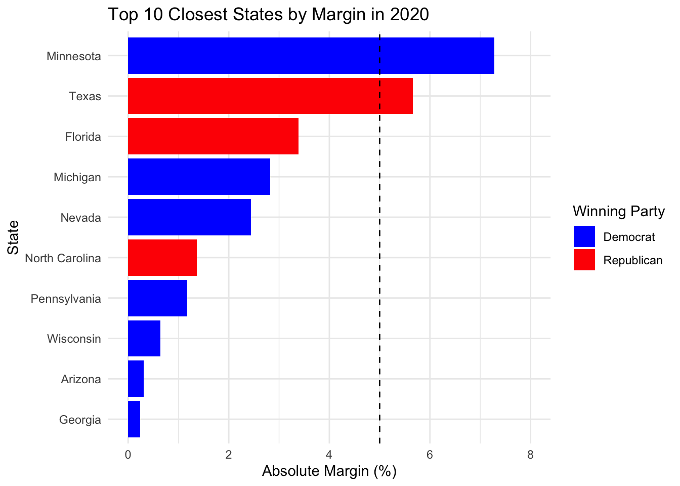
We drew a line at 5%. Here are the states where the margin is at most 5% in any of the past three elections.
##             state
## 1         Florida
## 2  North Carolina
## 3            Ohio
## 4        Virginia
## 5         Arizona
## 6           Maine
## 7        Michigan
## 8       Minnesota
## 9          Nevada
## 10  New Hampshire
## 11   Pennsylvania
## 12      Wisconsin
## 13        Georgia
Another way of measuring competitiveness is whether a state does not have the same winning party in the past three elections. This can be different from above if for example the entire state swung by more than 5% in each election.
## [1] "Arizona"      "Florida"      "Georgia"      "Iowa"         "Michigan"
## [6] "Ohio"         "Pennsylvania" "Wisconsin"
Iowa is one such state that swung very hard. I will add it to the list of competitive states.
Now we can run our model for each of the 14 states by introducing factors for each state. This will give us one model but in effect as if we had 13 models, one for each state.
## LOO-RMSE (Q3 GDP, September approval, competitive states, total): 10.67901## LOO-RMSE (Q3 GDP, September approval, competitive states, non-incumbents): 6.974695Putting in state indicators to predict state-level popular vote share increased LOO-RMSE from 6.27 to 10.7, and for non-incumbents from 4.5 to 7.0.
For an illustrative example, let’s look at how well the model predicts the popular vote share for Pennsylvania (leaving that year’s data out)
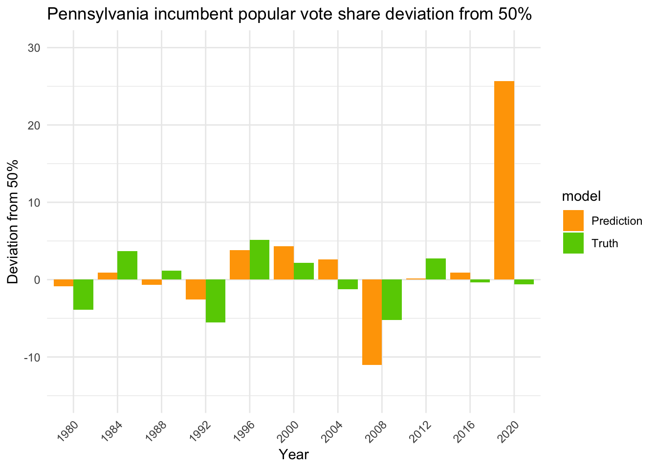
Again, there is the 2020 COVID outlier. Let’s remove it and see how our model performs.
## LOO-RMSE (Q3 GDP, September approval, competitive states, no 2020, total): 7.464242## LOO-RMSE (Q3 GDP, September approval, competitive states, no 2020, non-incumbents): 7.449431The LOO-RMSE for all elections decreased from 10.7 to 7.5, while for non-incumbents it increased from 7.0 to 7.4. Here’s the plot for Pennsylvania again.
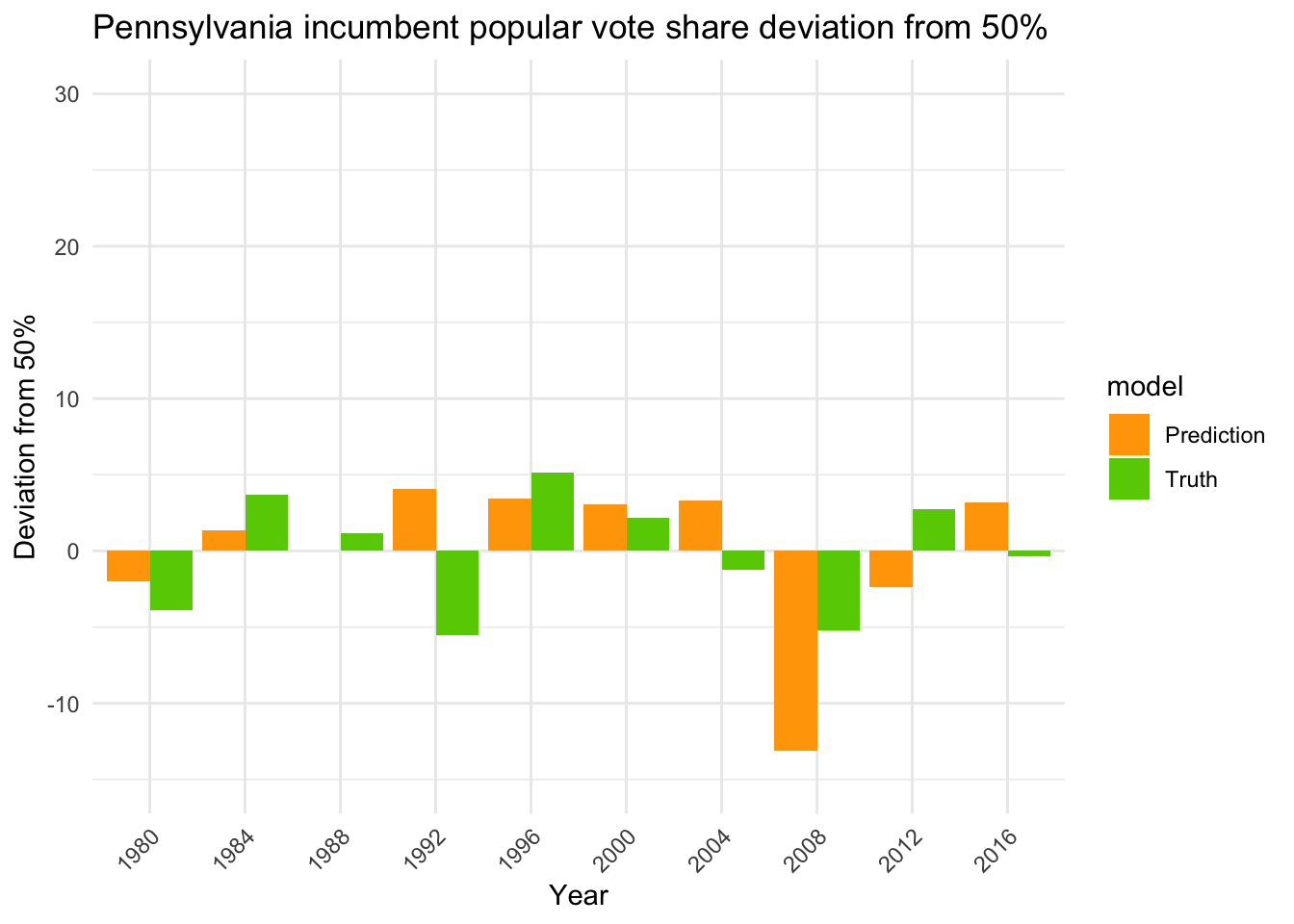
It might be possible that the linear model is not powerful enough under our setup to express partisanship in states. Let’s use the more powerful random forest.
## LOO-RMSE (Q3 GDP, September approval, competitive states, no 2020, total): 6.944223## LOO-RMSE (Q3 GDP, September approval, competitive states, no 2020, non-incumbents): 6.530832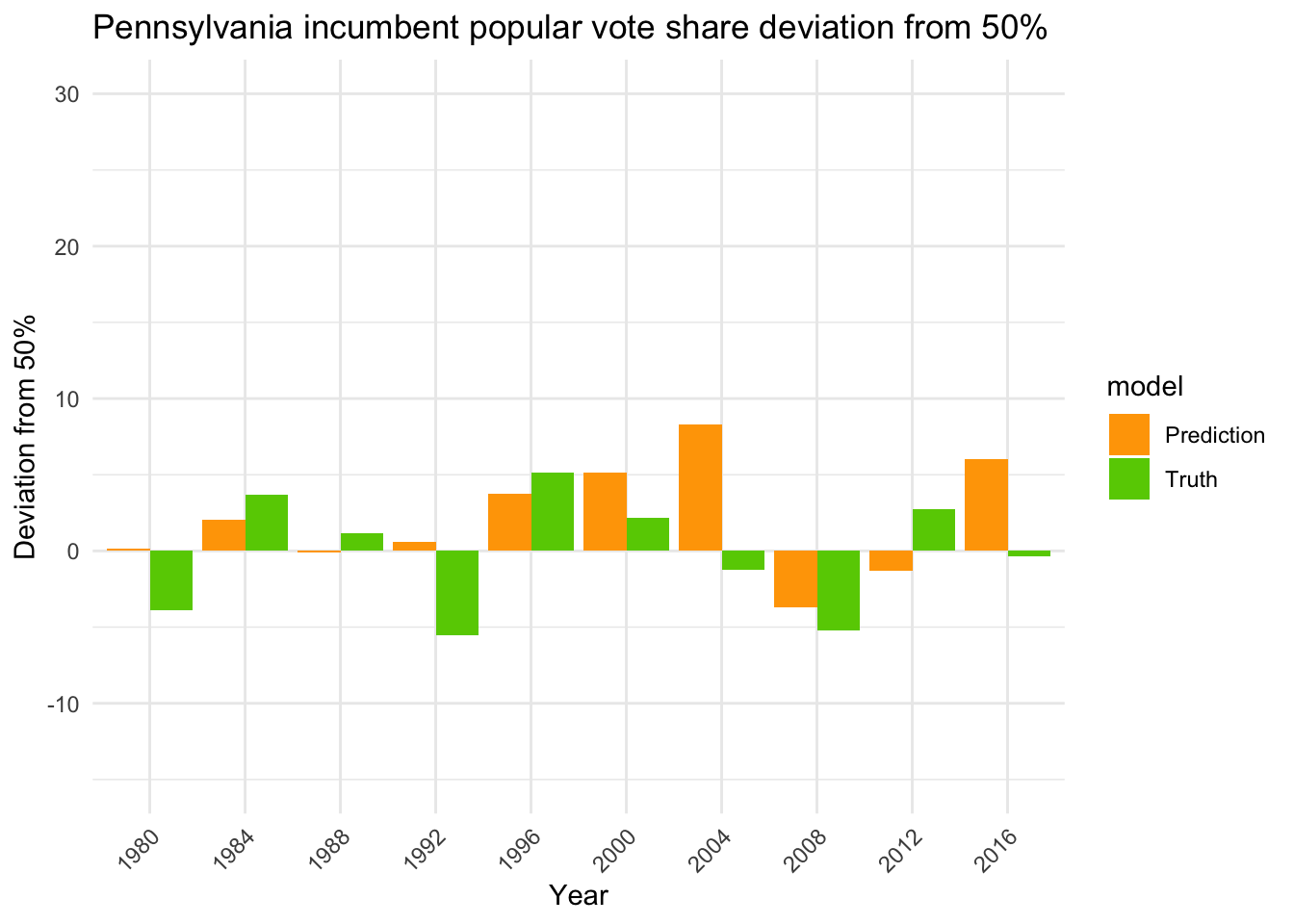
The LOO-RMSE for all elections decreased from 7.5 to 6.9, while for non-incumbents it decreased from 7.4 to 6.5.
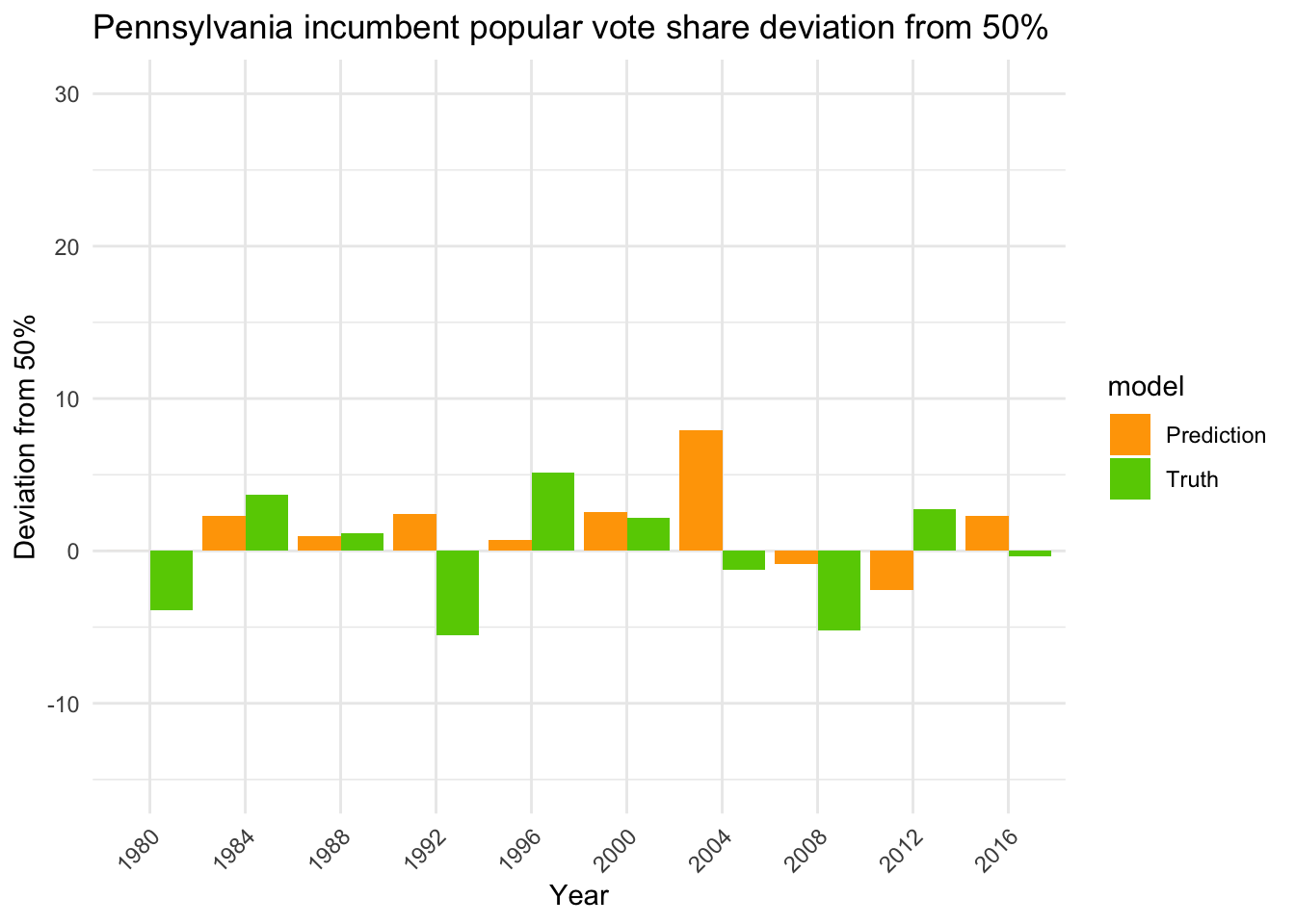
Let’s try to include partisanship into the data, by including whether the incumbent party is Democrat or Republican.
## LOO-RMSE (Q3 GDP, September approval, competitive states, no 2020, total): 6.685954## LOO-RMSE (Q3 GDP, September approval, competitive states, no 2020, non-incumbents): 5.214889The LOO-RMSE for all elections decreased from 6.9 to 6.7, while for non-incumbents it decreased from 6.5 to 5.2.
Campaign Contributions
Here are some data on the geographic source of campaign income of both parties for the past three elections.
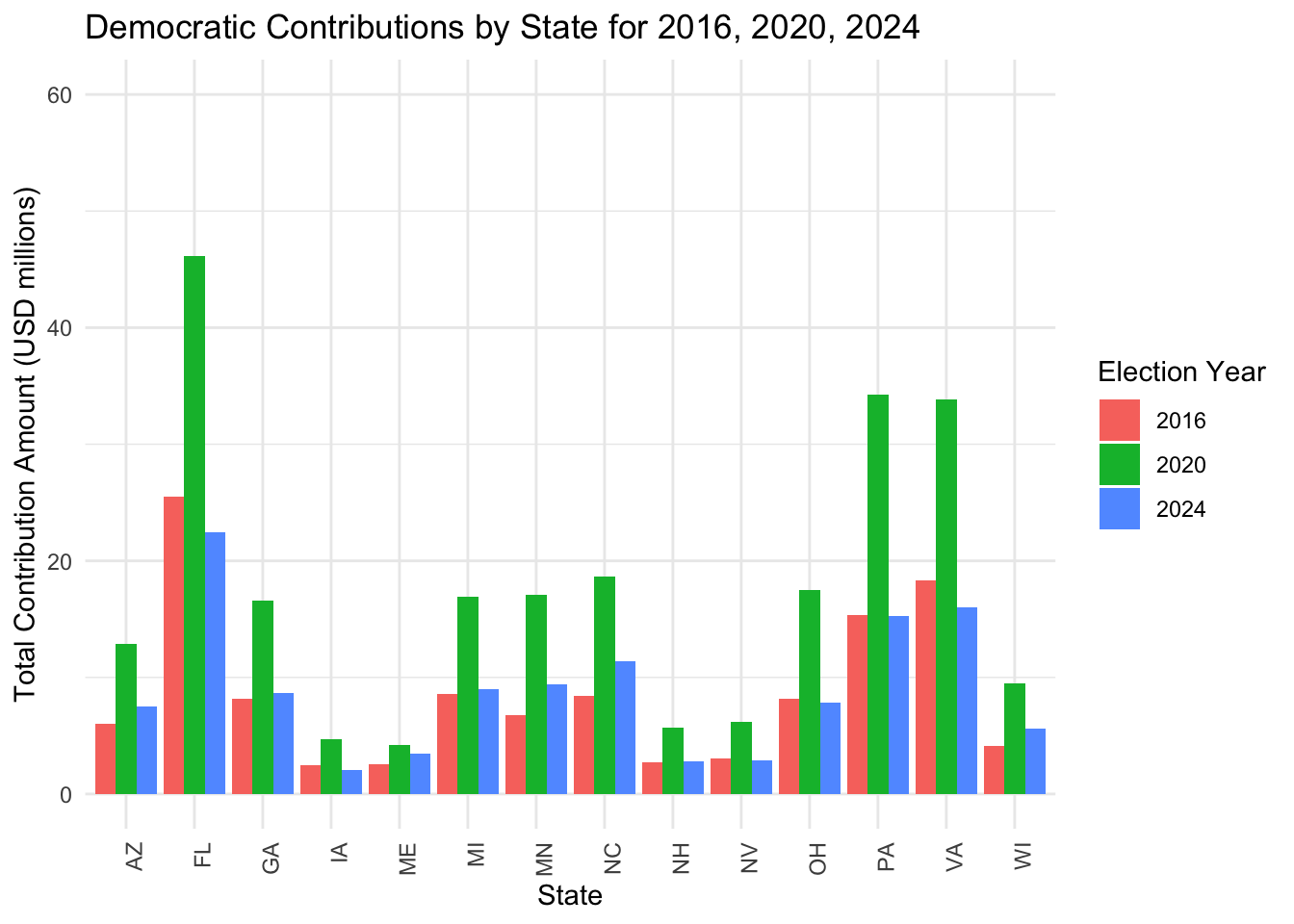
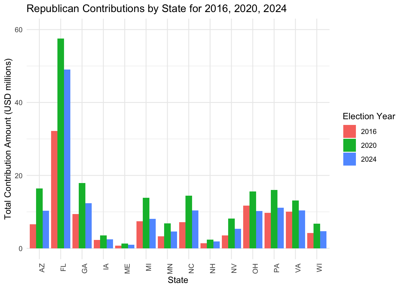 We can see that in these competitive states, campaign contributions are similar.
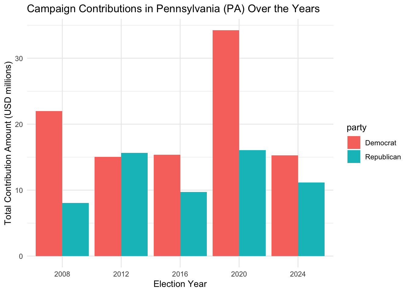
Let’s investigate if we can use campaign contributions to help forecast the vote share of the state. Here we only have data from the 2008, 2012, 2016 and 2020.
## LOO-RMSE (Q3 GDP, September approval, competitive states, 2008-2020, campaign contributions, total): 3.926477## LOO-RMSE (Q3 GDP, September approval, competitive states, 2008-2020, campaign contributions, non-incumbents): 4.183761Let’s compare it to our previous model if we only evaluate on 2008 to 2020.
## LOO-RMSE (Q3 GDP, September approval, competitive states, 2008-2020, total): 3.651691## LOO-RMSE (Q3 GDP, September approval, competitive states, 2008-2020, non-incumbents): 3.822718It seems like introducing campaign contributions doesn’t help with predictions, so we will discard campaign contributions going forward. One thing we could look into, is campaign spending on each state. We would like to do investigate that if we have the data.
One last step before we finalize a working model: limit the scope of our training data. The rationale is that data from older elections might not be useful in forecasting future elections. Here we calculate the LOO-RMSE if we train the model with data starting from that date
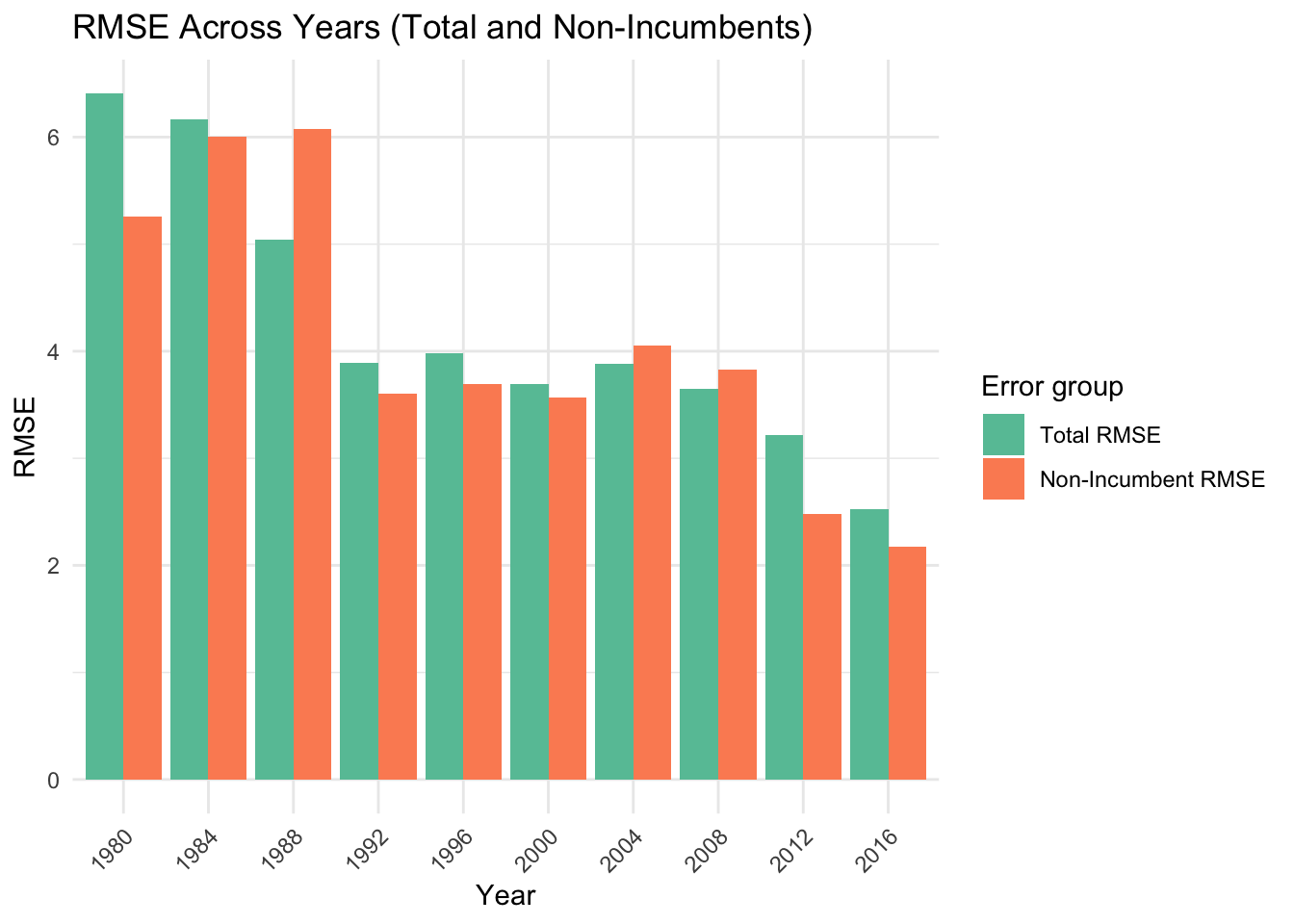
The plot above motivates using 1992 onwards.
Final working model
We predict the incumbent party two-party vote share of a state using random forest model given the following data
- Q3 GDP growth
- Gallup September presidential job approval rating
- whether the incumbent party candidate is themselves an incumbent
- State
- whether the incumbent party is the Democrat Party
We train it on data from 1992 to 2020. This model achieves a LOO-RMSE of
## LOO-RMSE (total): 3.877684## LOO-RMSE (non-incumbents): 3.631876The model predicts the following for 2024.
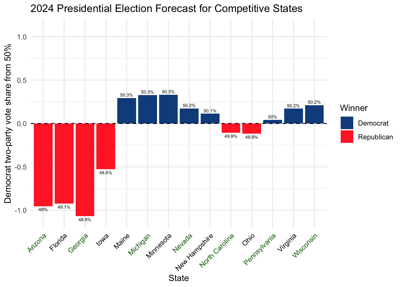
Toss-up states are labelled in green (see our blog on expert predictions for identifying toss-ups).
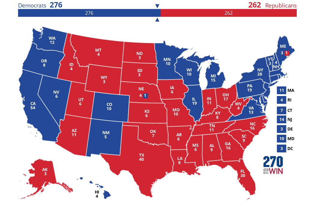
I would like to point out that the model predicts a close race for the non-swing states New Hampshire and Ohio, but the model agrees on the winner with expert predictions on these non-swing states. Be careful that the model has a LOO-RMSE of 3.68 for the 2024 situation, while all the states forecasted here are within 1% from 50%. The model predicts a Harris win with 276 vs 262.
The next step will be to quantify uncertainty and answer this question: if we run a simulation with our model 1000 times, how often will Harris win?
