The code for this page can be found here.
One measure of the economy is the GDP growth. But do voters care more about the short-term GDP growth in the months leading up to the election, or do they judge the candidate based on the GDP growth throughout their term? We first investigate the Q2 GDP growth, which is by how much did the GDP grow in the second quarter (April, May, June) in the year of the election.
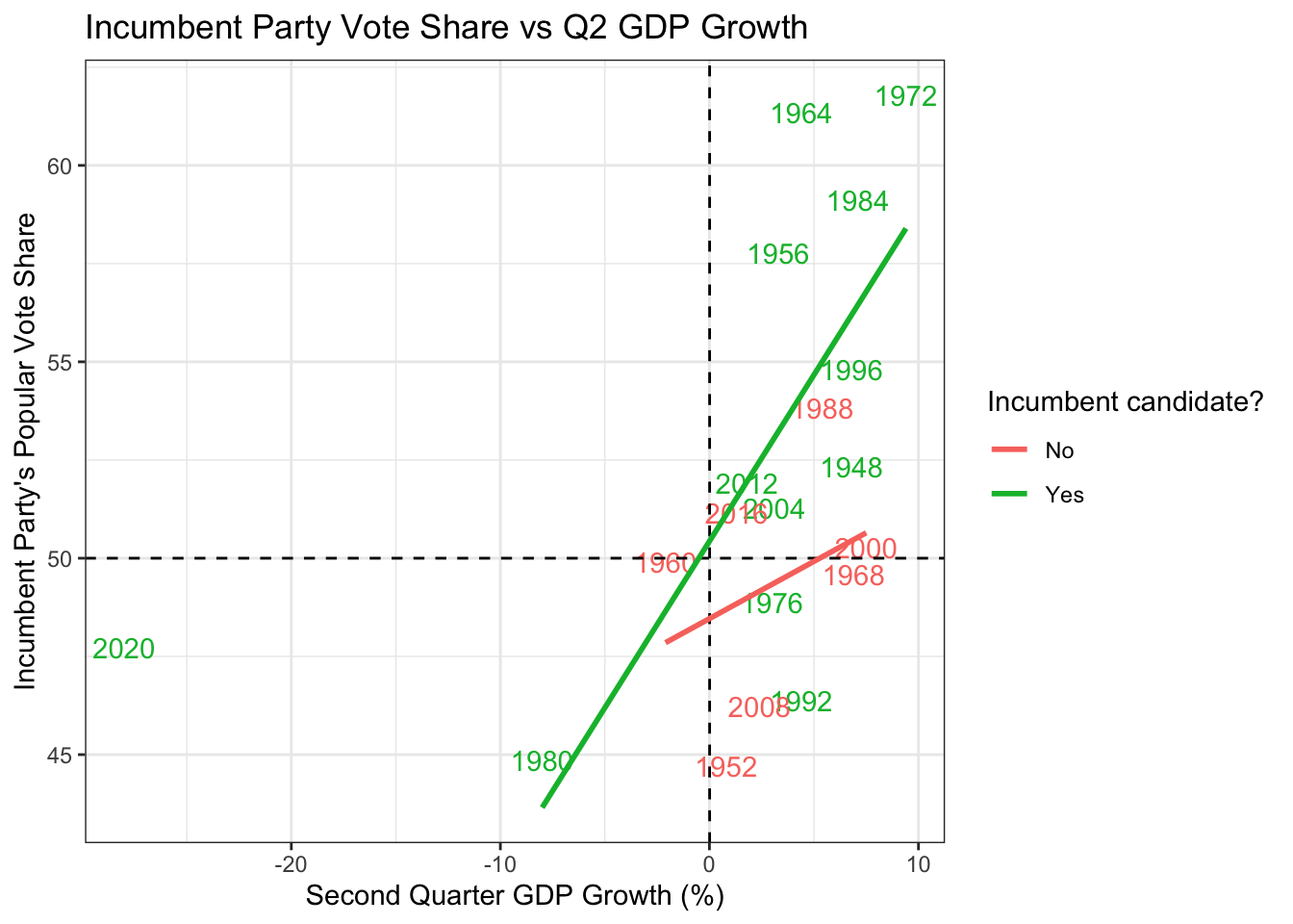
In our best-fit lines above, we have removed 2020 as an outlier. The plot shows that there is a strong positive correlation between second quarter GDP growth and the incumbent’s party vote share, particularly so when the candidate is also incumbent! This is fair, since the voters might not judge a new non-incumbent candidate with the current economy. Another interesting feature is that the best-fit line almost cross the center of 50% vote share for 0% growth. This suggests that the voters only reward the incumbent with more votes if the economy grows, and punishes when not, with no established baseline that the president is expected to perform. Let’s look at the \(R^2\) to get an idea of how powerful is the prediction. Here’s the \(R^2\) for non-incumbent candidates.
summary(lm(pv2p~GDP_growth_quarterly,
           data=(d_inc_econ|>filter(incumbent==FALSE))
           ))$r.squared
## [1] 0.1142466Here’s the \(R^2\) for incumbent candidates.
summary(lm(pv2p~GDP_growth_quarterly,
           data=(d_inc_econ|>filter(incumbent==TRUE, year!=2020))
           ))$r.squared
## [1] 0.4373633It turns out that second quarter GDP growth can explain up to 44% of the change in vote shares across time! Now, how about long term GDP growth? Instead of looking at the GDP growth during the election year, let’s compare the GDP growth from the start of their term to the end of the term.
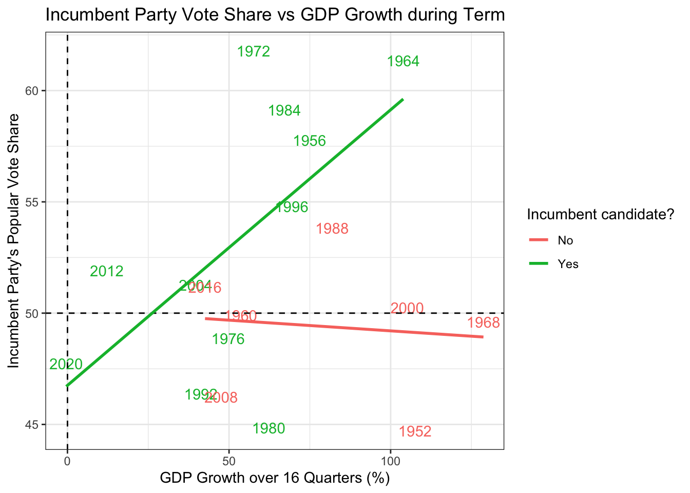
Here’s the \(R^2\) for non-incumbents.
summary(lm(pv2p~GDP_growth_termly,
           data=(d_inc_econ|>filter(incumbent==FALSE))
           ))$r.squared
## [1] 0.01141712Here’s the \(R^2\) for incumbents.
summary(lm(pv2p~GDP_growth_termly,
           data=(d_inc_econ|>filter(incumbent==TRUE, year!=2020))
           ))$r.squared
## [1] 0.2929693Interestingly, the effect on non-incumbent candidates essentially flattens out. Voters do not judge new candidates based on how well the economy performed over the years. For incumbent candidates, we still see a strong positive correlation, but the explanatory power decreases from 44 to 29. This suggests that the short-term national economy has more influence on elections that the long-term trajectory. Another interesting feature is that the best-fit line crosses the 50% mark when the GDP growth is 29.6%. This means that in contrast to the second-quarter GDP growth, the voters impose a baseline performance for the president to sustain the growth of the economy.
How about other measures of the economy like unemployment rate? Here we took seasonally-adjusted unemployment rate for each state and see if the vote share of the incumbet party in each state changes in response to the unemployment rate.
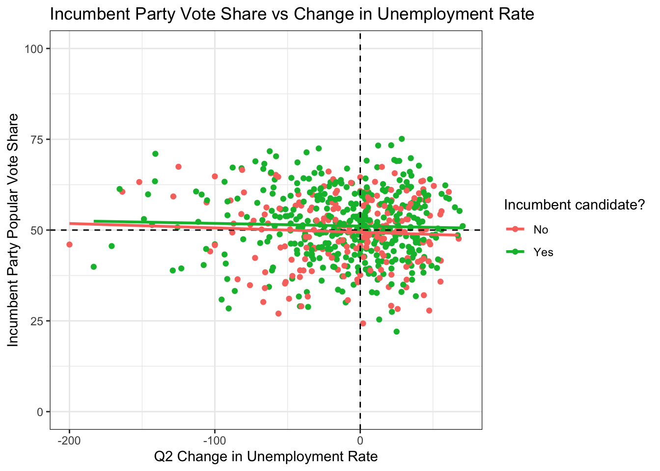
Here’s the \(R^2\) for non-incumbents.
summary(lm(pv2p~q2_unrate_growth,
           data=(d_unrate_enc|>filter(incumbent==FALSE))
           ))$r.squared
## [1] 0.003274093Here’s the \(R^2\) for incumbents.
summary(lm(pv2p~q2_unrate_growth,
           data=(d_unrate_enc|>filter(incumbent==TRUE, year!=2020))
           ))$r.squared
## [1] 0.0005243959The flat line and low \(R^2\) in both cases suggest that unemployment rate does not have a huge say on who becomes president. This suggest that voters do not associate employment with the president, since they might see more as a personal matter.
Let’s put all the economic indicators we have into a machine learning model and see which indicators are most effective in predicting the national vote share. We build a random forest model with 100 trees and look at the importance plot which shows how good each indicator is in predicting vote share.
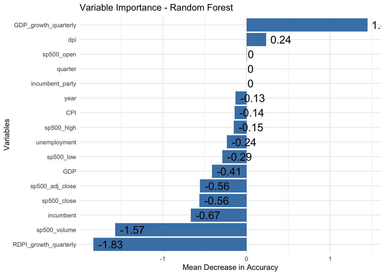
The random forest confirms our hypothesis and crowns the second quarter GDP growth as the strongest economic predictor of the election, followed by the S&P 500 open and the incumbency effect. Let’s use these three predictors to predict the next election and check the leave-one-out cross-validation (LOO-CV) error.
## [1] "LOO-CV Mean Squared Error: 25.5103785768594"## [1] "LOO-CV Root Mean Squared Error: 5.05077999687765"The RMS is 5.05 which can be interpreted as saying that the prediction is usually within 5% of the truth. Let’s use this model to predict the current election.
set.seed(1347)

data2024 <- d_fred|>filter(year==2024,quarter==2)
data2024$incumbent <- FALSE

rf_model <- randomForest(pv2p ~ GDP_growth_quarterly + sp500_open + incumbent,
                           data = d_inc_econ, ntree = 100)

predict(rf_model, data2024)
## 1
## 49.83405The model suggests a vote share of 49.8% for Kamala Harris using GDP growth rate, S&P 500 and the fact of non-incumbency. It can be interesting to note that the economic indicators itself are on the fence in this election and not particularly strong. Even if an incumbent runs, the vote share is 50.7%.
data2024 <- d_fred|>filter(year==2024,quarter==2)
data2024$incumbent <- TRUE

rf_model <- randomForest(pv2p ~ GDP_growth_quarterly + sp500_open + incumbent,
                           data = d_inc_econ, ntree = 100,)

predict(rf_model, data2024)
## 1
## 50.71584Since the economic indicators are not vocal, both Harris and Trump have no edge in terms of the economy.